On November 6 2015, I was asked to give a talk at BLUE1647, a Chicago technology center, on some of the projects I worked on while at Quantopian. Below are the slides from the talk, as well as the (approximate) transcript.
Thank you for joining me tonight! My name is John Loeber, and my presentation will be in two parts, based on work I recently did at Quantopian. For the first part, we'll discuss an implementation of the Fama-French Factors using the Pipeline API, which Quantopian released just a few weeks ago. For the second part, I'll showcase Quantopian's research platform, and use naive parameter optimization to find out whether lay investors should sell off their assets when the market turns.
For our discussion of the Fama-French Factors, we'll briefly go over factor models.
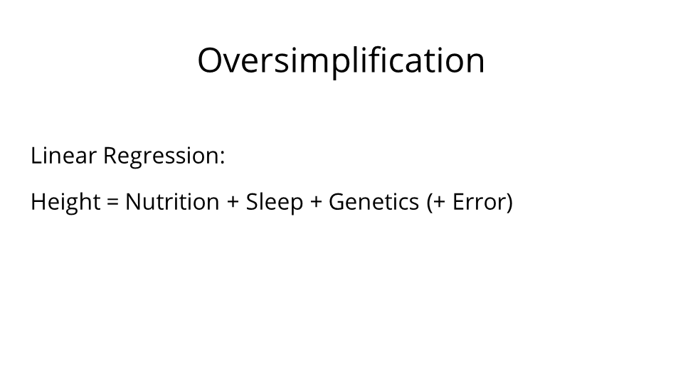
To start: what's a linear factor model? Well, it's a linear regression model. You try to predict a variable given a set of variables to regress against. In this example, we say that someone's height can be predicted or described by a combination of three factors: nutrition, sleep, and genetics — plus some term that accounts for a bit of random error.
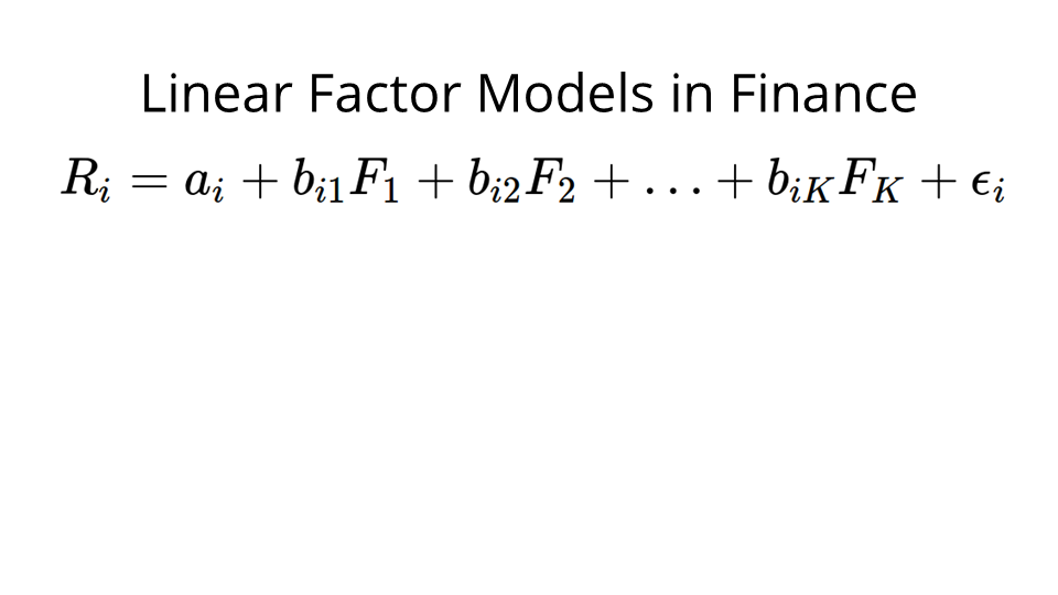
More formally, in finance, a linear factor model looks like this. We try to predict or describe the returns of an individual security, Ri, using a combination of factors.
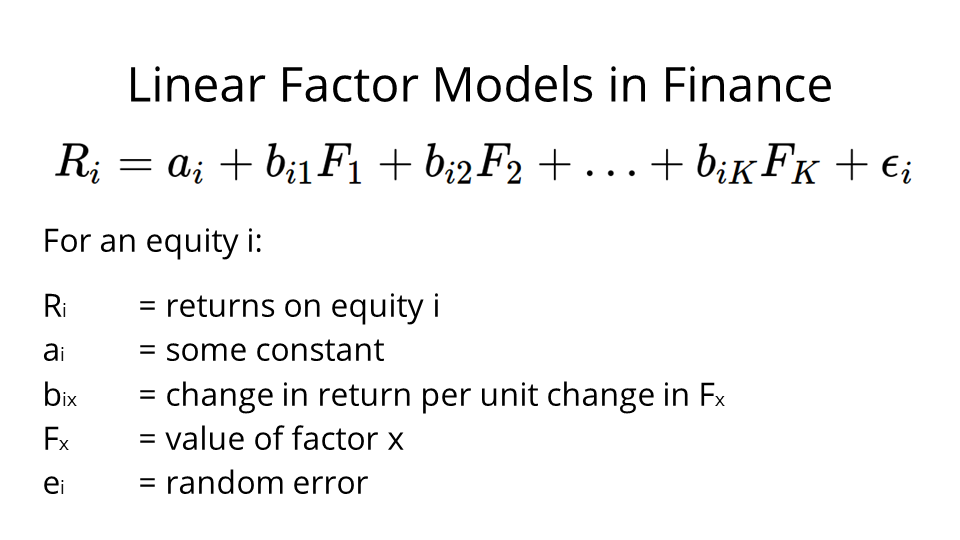
So for an equity i, we describe the returns using this linear combination: we've got a constant term, ai, then we have a bix coefficient for each one of our factors. We have the factors themselves — the Fx, and again, a random error term in the end, because no prediction is going to be perfect.
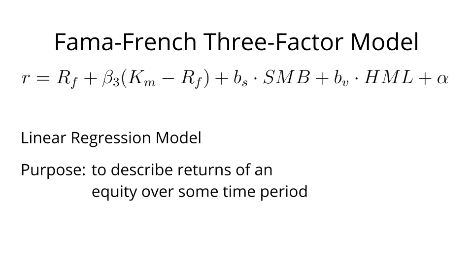
With that covered, here we have the Fama-French Three-Factor Model. Again, it's a linear regression model to describe security returns over some time period.
To explain: the idea here is that stock returns, over some time period, can be described by three factors, which follow three central observations.
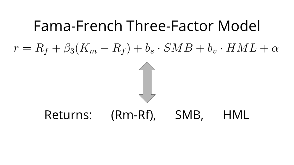
- The first observation is that the returns of the market are generally effective in describing the returns of a single stock. Thus, Rm minus Rf is the returns of the market minus the risk-free rate of return.
- Secondly, Fama and French noticed that small cap stocks generally tend to outperform large cap stocks, so SMB is the returns of small cap stocks minus the returns of large cap stocks.
- Third: Fama and French were also of the opinion that value stocks outperformed growth stocks, so HML is the returns of stocks with a high book-to-market ratio (value stocks) minus the returns of those with a low book-to-market ratio (growth stocks).
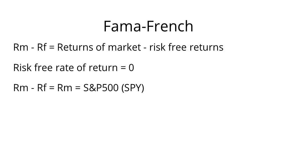
In our implementation, we don't really believe in risk-free returns. So Rm minus Rf is just going to be Rm, represented by SPY, which is Standard & Poor's 500 Index.
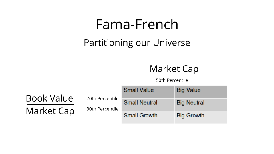
To get SMB and HML, we'll want to partition our universe of securities into six categories as such. We'll then want to get the returns of each of these six categories.
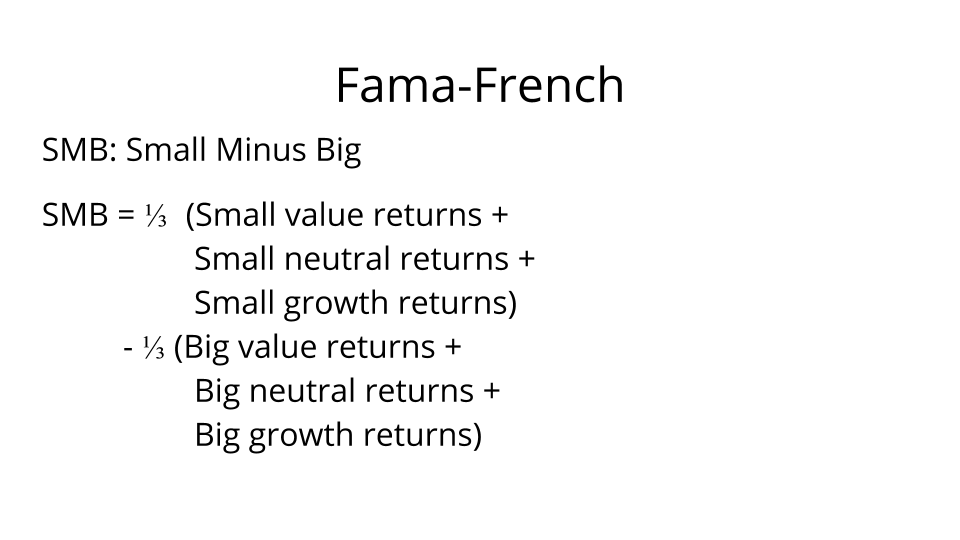
Once we have those returns, we can use them to compute our factors. Here's how we compute SMB.
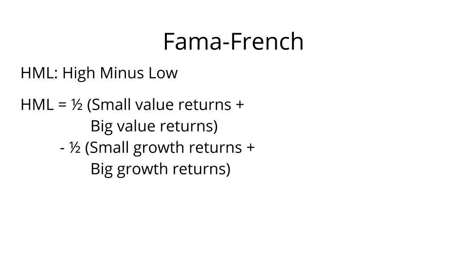
And here's how we compute HML.

Thus, quite straightforwardly, computing these factors only requires us to partition our entire universe of securities, grab the returns of the partitions, and then do some arithmetic. But working with a large universe of securities is technologically not trivial.
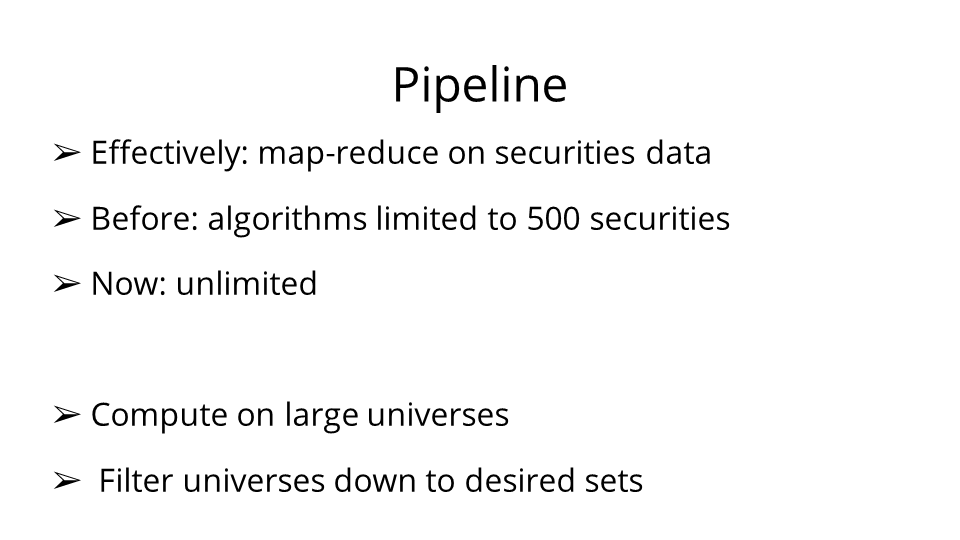
And that's why Quantopian released the Pipeline API a few weeks back. Conceptually speaking, Pipeline lets you work with the entire Quantopian universe — well over 8000 securities — in a kind of map-reduce way. You can map operations over every single security and its corresponding pricing dataset at once. In turn, you can compose these operations to get essentially any datastream you can possibly derive from the data. Furthermore, you can use these operations to create filters, thereby filtering your universe down to the equities you want according to your criteria.
Thus, this technology — which, by the way, is the only one of its kind that is freely accessible to the public — is extremely powerful.
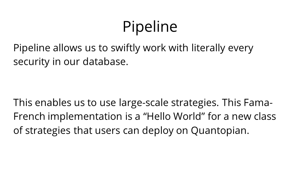
To summarize: Pipeline allows us to work swiftly and highly effectively with every security in our database. This creates enormous opportunities for users, chiefly enabling them to use large-scale strategies. In that sense, this Fama-French implementation is a kind of “Hello World” to showcase an entirely new class of strategies and investigations that users can carry out on Quantopian.
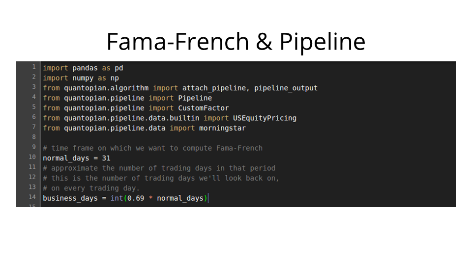
So let's talk about the implementation in detail. How's the code? Well, we import our libraries and then decide on the window length over which we want to compute rolling Fama-French factors.
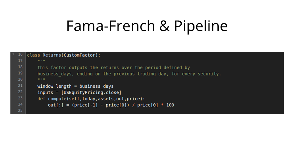
We create a factor for returns over the time period. It'll map every security to its returns at the end of the period.
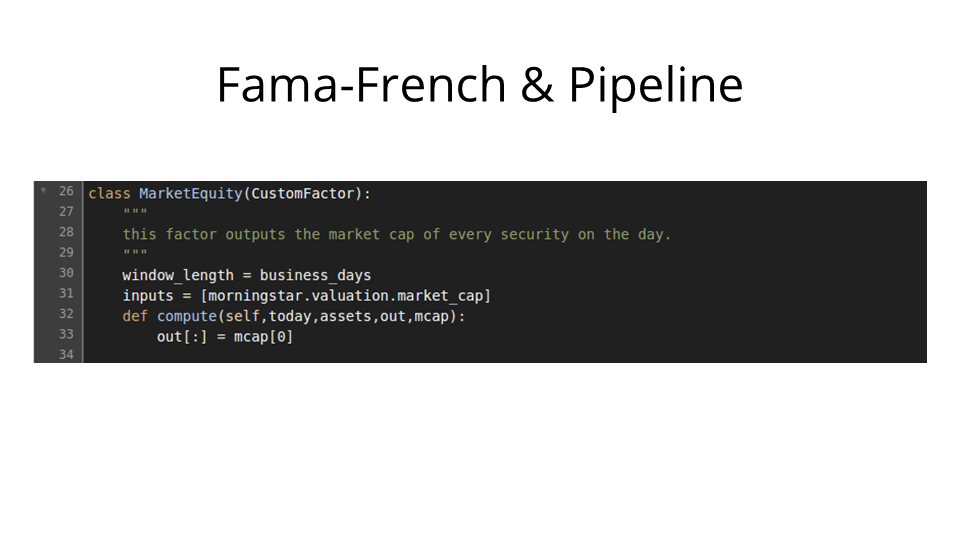
Next, we create a factor that gives us the market cap of every security at the start of the period.
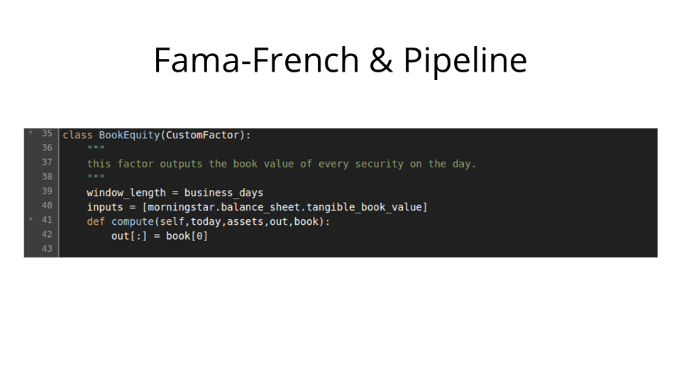
We create a factor that gives us the book value of every security at the start of the period.
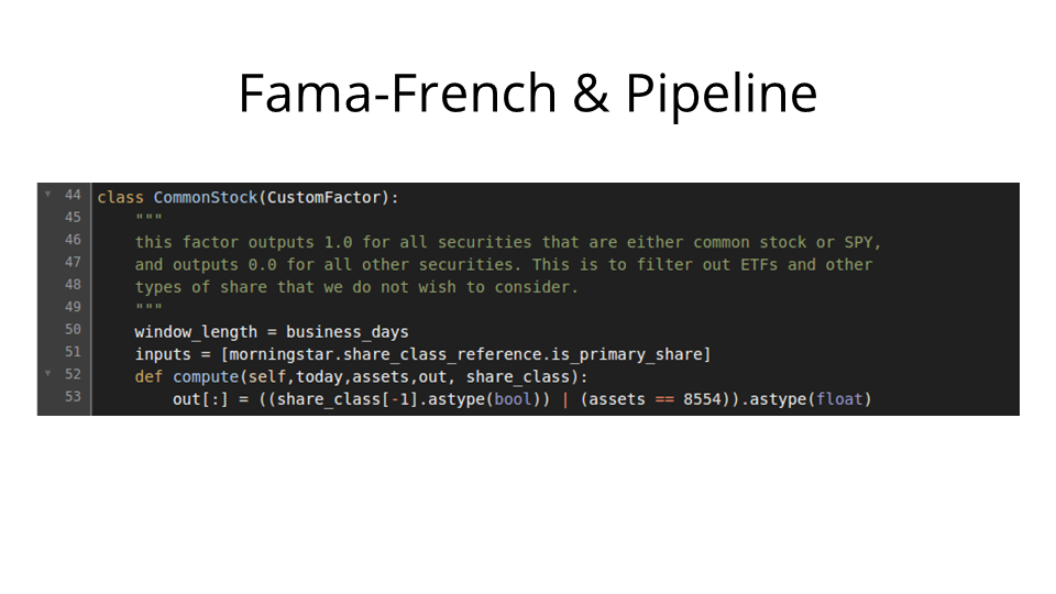
We create a factor that outputs one or zero depending on whether or not a security is a common stock or SPY, or not. This is so we can filter the universe down to common stock and SPY only. We'll need SPY since it is our benchmark.
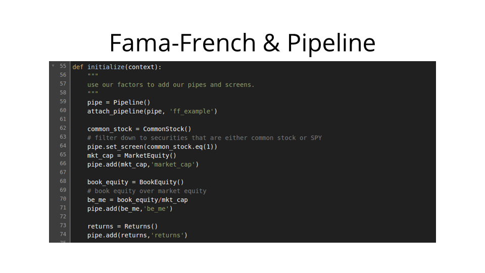
In initialize — this section only runs once at the very beginning of our algorithm — we add all our pipes, set the screen — that is, the filter — and create the book equity over market equity pipe. Note that it's as simple as literally dividing the book equity pipe by the market equity pipe.
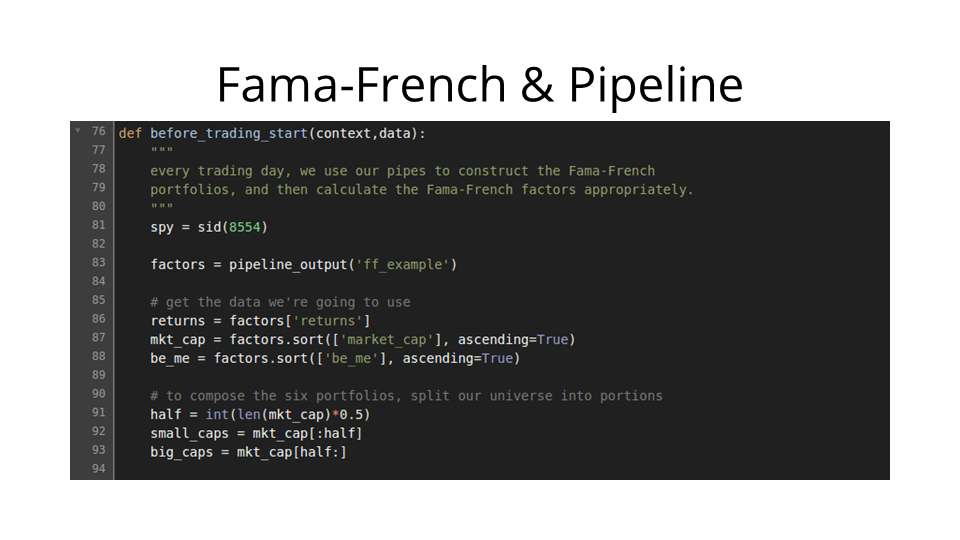
I've put the main logic into before_trading_start. We get our three factors: returns, market cap, and book equity over market equity. We get the 50th percentile, and appropriately partition our universe into small caps and large caps.
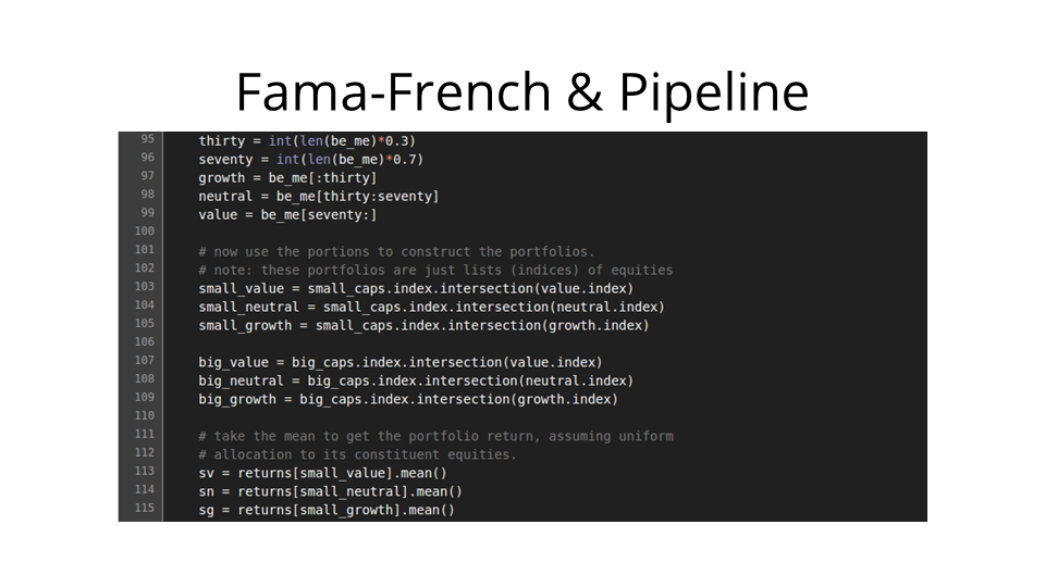
We then partition our universe into the growth, neutral, and value portfolios. We then intersect these three portfolios with the small-cap and large-cap portfolios in order to split our universe into the six desired portions. At the bottom, we get the returns for the three small portfolios.
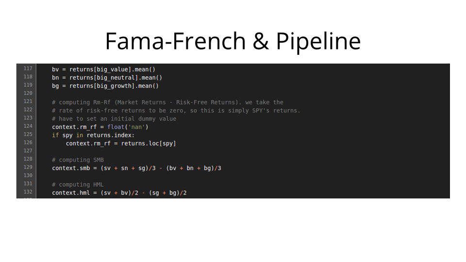
Next, we get the returns for the three big portfolios, grab the return of SPY, and do some simple arithmetic to find SMB and HML.
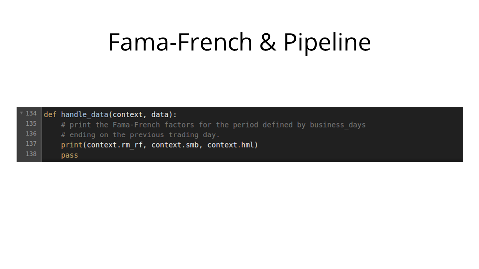
Then we just print the three-tuple (RM, SMB, HML) on every trading day.
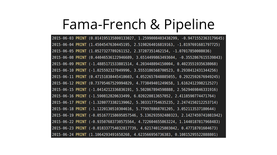
And the output in the algorithmic trading IDE looks like this. We can then export it to a spreadsheet with relative ease.
Next up, you might ask: how good is our implementation of Fama-French?
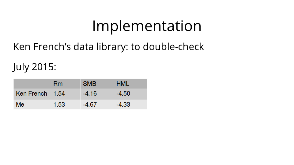
Thankfully, Ken French actually computed the Fama-French Three Factor Model for a significant number of various time periods, and placed these canonical values on his website. So I was able to compare my results to his. Here is a comparison for July 2015.
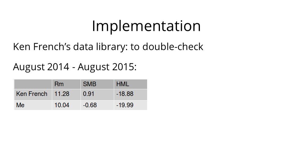
And here are the results for August 2014 through August 2015.
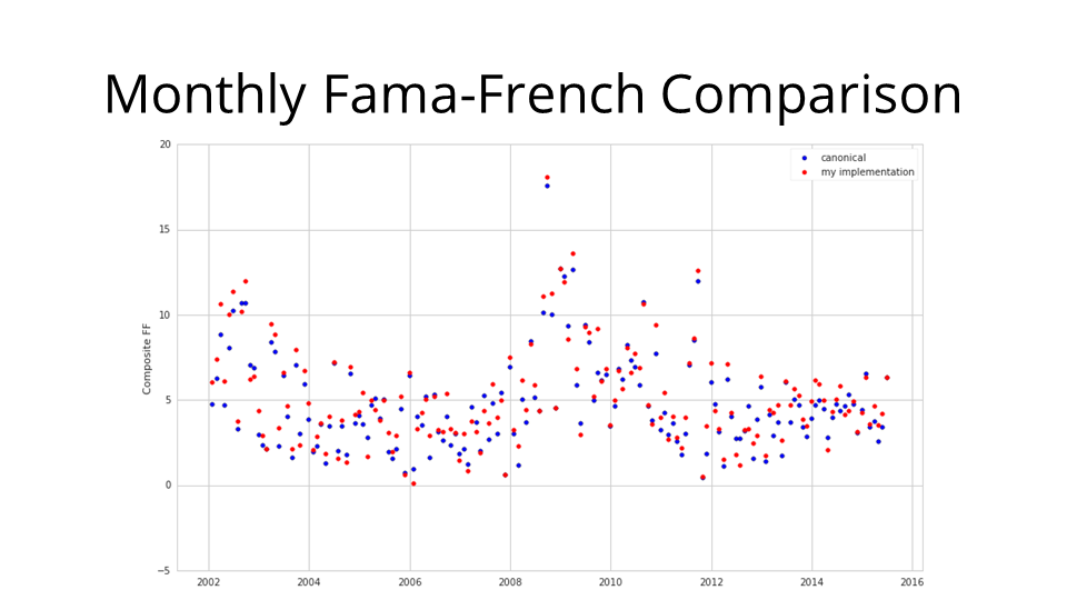
I then used some dimensionality reduction techniques to conduct a more general comparison: here's a plot of the three Fama-French factors combined into one metric for every month over the last thirteen and a half years: blue are canonical, red are mine. We generally see that they're quite similar.
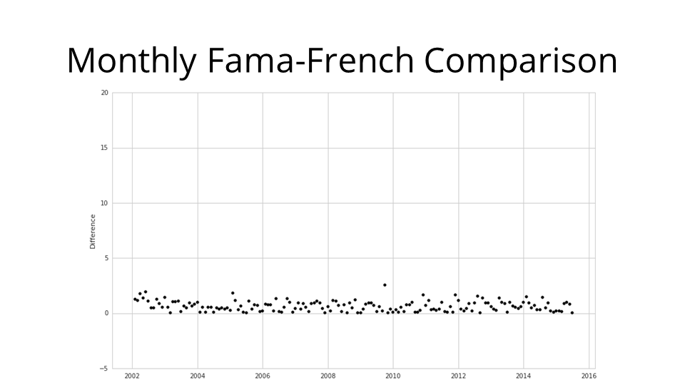
But of course there are some differences. Much of these differences is due to methodology: Ken French computes his factors over calendar months, but the native unit on Quantopian really is the trading day, so I computed these factors over periods of trading days, rather than calendar months. Making sure that all my periods line up with those of Ken French was somewhat challenging.
Moreover: the canonical Fama-French factors published by Ken French only rely on three exchanges: AMEX, NYSE, and NASDAQ. Quantopian pulls in data from over twelve US exchanges. Consequently, this implementation arguably offers a more holistic and complete view of the factors.
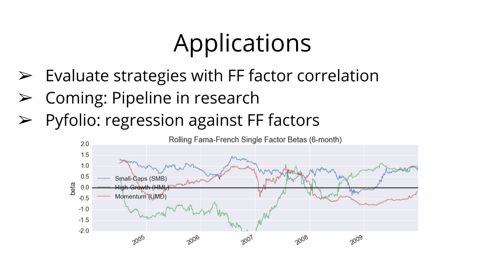
So: what are the applications of this? How can we use the Fama-French factors to generate alpha? Well, we usually use them to evaluate the performance of a trading strategy. Specifically, in the pyfolio library, which was developed and open-sourced by Quantopian, users are encouraged to look at six-month rolling Fama-French factors, and to correlate those factors with the returns of their strategies. The reason for this is that it often happens that someone may think they're trading on some particular signal, but a correlation analysis shows that 95% of that signal is explained by SMB.
Once the Pipeline API comes to Quantopian's research environment, users will be able to use this implementation to generate, modify, and work with Fama-French factors over any rolling time window. I expect that this will add yet another powerful tool for users to evaluate and prime their strategies.

Now that we're talking about the research environment, let's move on to the next project: using naive parameter optimization to investigate strategies for lay investors.
As a recap: Quantopian's research environment is an iPython platform on which you can run algorithms, import datasets, and use Python's data-analytic tools and libraries.
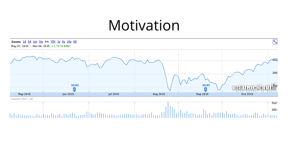
The motivation for this project was the small but scarily quick market downturn this August. This gave rise to a great flurry in the news: I saw many articles about whether people should sell off their assets when the market seems to turn, how effective people are at picking good times to sell and buy back, etc.
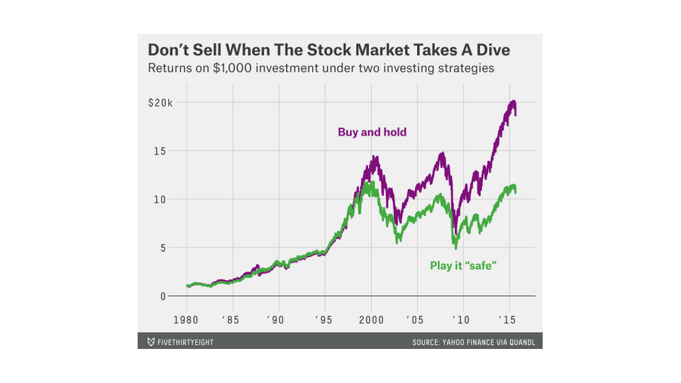
In particular, the folks at 538 published an article saying that investors shouldn't sell their stocks when the market turns. They simulated a strategy in which an investor sells every time the market loses five percent in a week, and buys back when it rebounds by three percent from its minimum since selling off. They made this cute graphic to drive home the point that people should simply hold on to their assets.
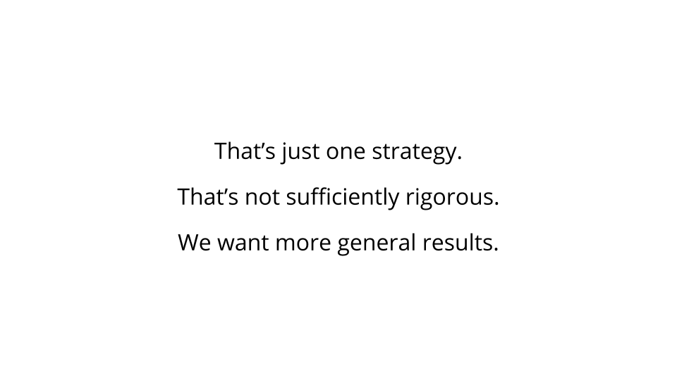
But that's not rigorous enough. A five-percent drop and three-percent rebound is only one configuration that someone might use. What about six percent and four percent? What about fifteen percent and five percent? Clearly, we want more general results.
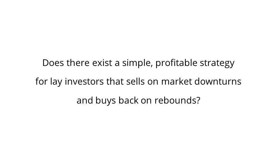
As such, my guiding question was along these lines: suppose that you're a lay investor. You don't really want to build a sophisticated strategy, short, hedge, or spend a great deal of time trying to figure out the markets. Suppose that you just want to look at the newspaper once a day, look at SPY values for the week, and plug that into your calculator. Naturally, one strategy in that vein is the simple drop-and-rebound strategy. We'll try to find the optimal drop and rebound percentages for selling and buying back. Note, by the way, that this is implicitly a mean-reversion strategy.
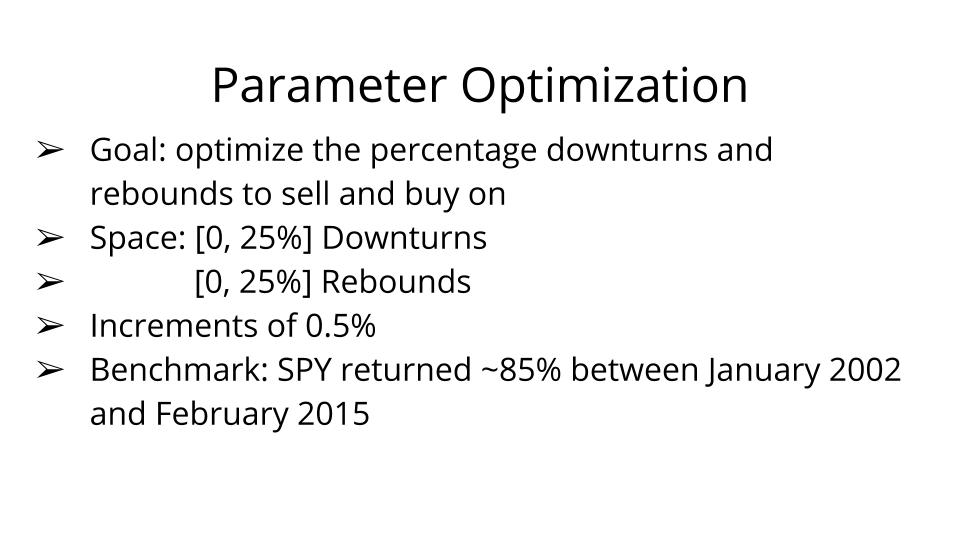
So, that's our goal. We'll go over this space of possible drops and rebounds in half-percent increments. In particular, we'll focus on strategies that beat the benchmark: SPY returned about 85% between January 2002 and February 2015.
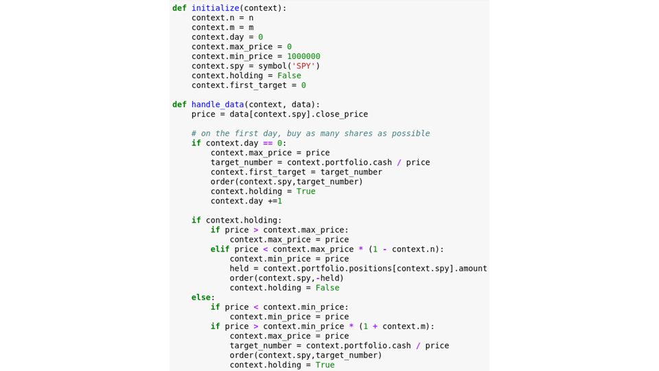
I wrote this very simple algorithm to sell or buy SPY as appropriate when SPY drops by m percent from a previous maximum, or rebounds by n percent from a previous minimum.
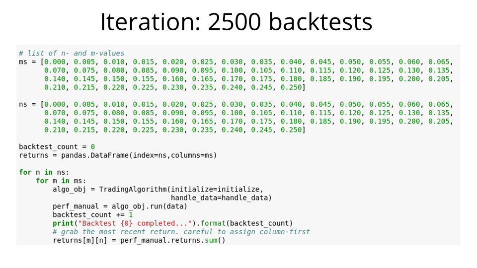
Next, I set up some code to iterate over all possible combinations for m and n, and for each combination, to run the algorithm and record the returns over the thirteen-year period.
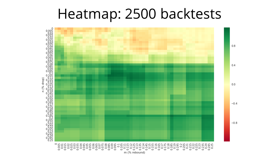
Running the 2500 backtests took a few hours, but the returns can be nicely visualized as a heatmap! We've got the rebound percent on the x-axis, and the drop percent on the y-axis.
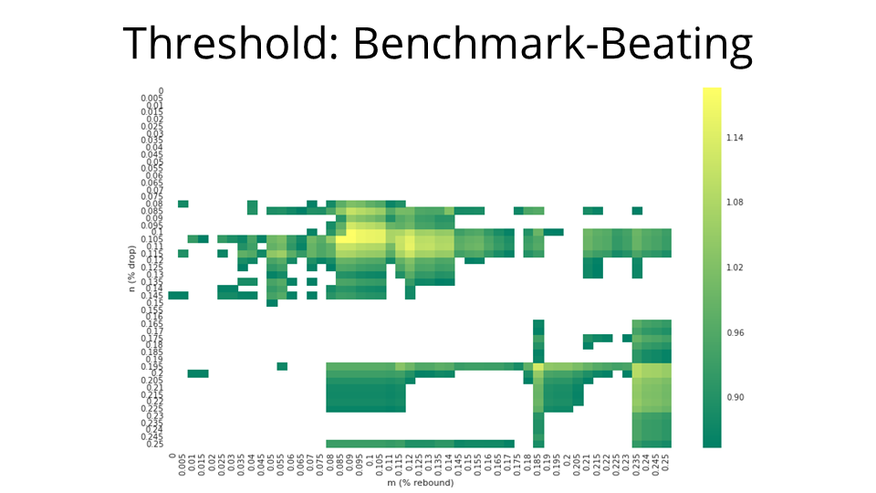
And we're really only interested in the benchmark-beating returns, so we filter the heatmap down to those (m,n) points that returned more than 85%. In this example, the best return is about 118.6%. That's a pretty substantial gain on 85%.
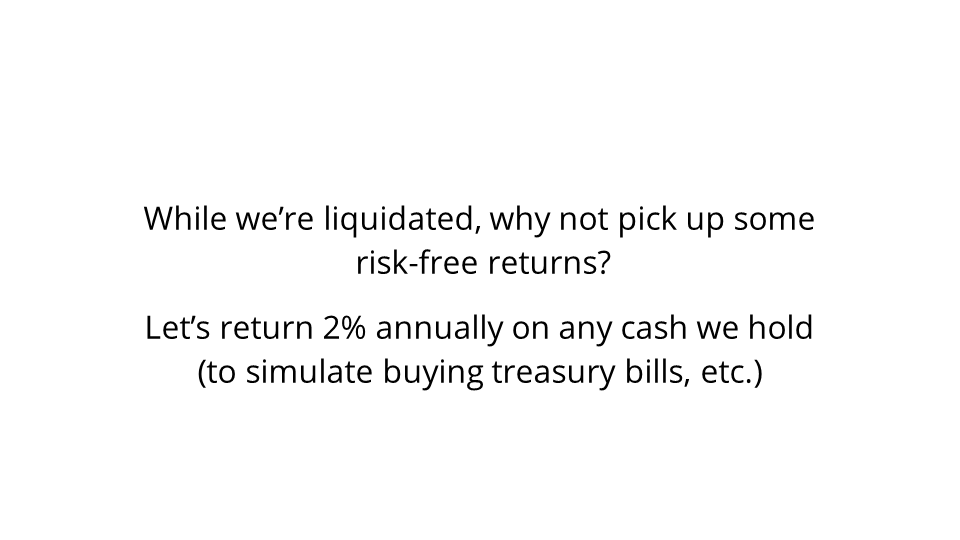
But this strategy does occasionally liquidate the entire portfolio and hold only cash. While that's the case, why not pick up some risk-free returns? I decided that while we're holding cash, we'll pretend to buy treasury bills or make a similar investment to return two percent annually — or about 0.008% per day. How does this affect our strategy? Let's run another 2500 backtests.
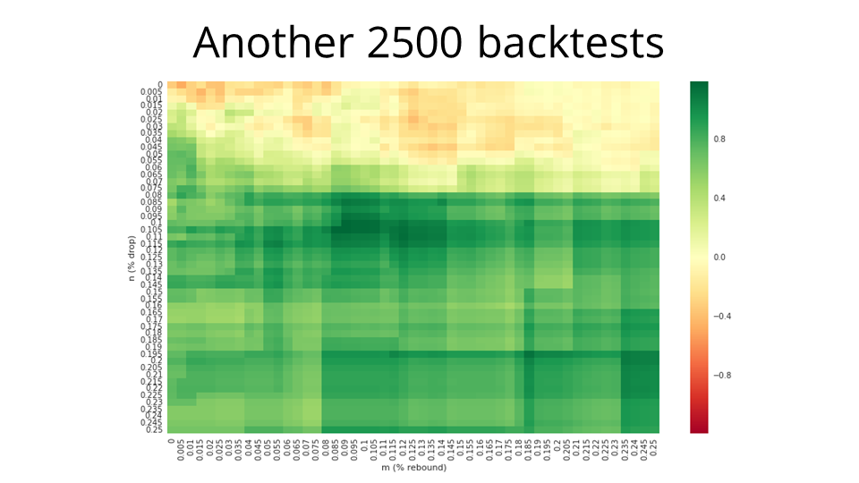
As it turns out, gaining about 0.008% per day compounded, for a relatively small number of days, doesn't make a particularly big difference. The heatmap looks effectively identical to the one we had before.
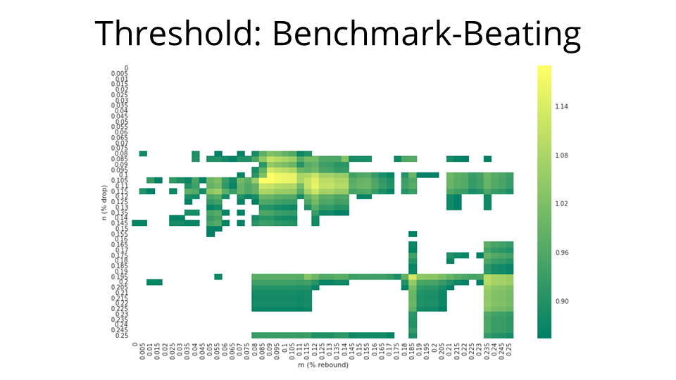
Again, we filter down to the benchmark-beating returns. The best return here is about 121.1%, which is marginally better than the 118.6% one from earlier. But now the big question is: can we rely on this strategy? I picked the optimal parameters — a drop of about 8.5% and a rebound of 10.5%, and ran a backtest.
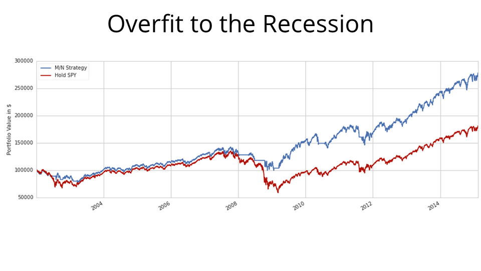
And in this backtest, we can see quite clearly that the reason this strategy was “successful” was that it was tremendously overfit to the recession. For the most part, SPY (in red) and the strategy (in blue) are totally commensurate in their movements, except for the recession. Around 2009, SPY drops like a rock, but our strategy sells off and holds cash. This means that when the markets began to recover, some time mid-2009, our strategy's portfolio is pure cash, worth about 50% more than the SPY portfolio. Then our strategy puts all its cash in SPY. Then we have two portfolios: one of them consists of 100k in SPY, the other consists of 150k in SPY. Five years of bull-market compound growth later, it stands to reason that the cash difference is exaggerated and one of them is worth far more than the other.
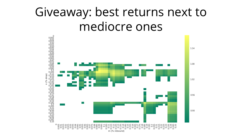
Back to this heatmap. For the entire bubble in the middle, the behavioral pattern is exactly the same. All of these (m,n) strategies are effectively calibrated to stop out in a very narrow one or two week window, just avoiding the worst of the recession, and then they all buy back in the same one-or-two week window a few months later.
The real dead giveaway that we've got a colossal overfit here is that we have the point with the best possible returns almost adjacent to points with mediocre returns and ones that fail to beat the benchmark. That's for tiny differences in m and n. Sub-percent calibrations should not make that kind of difference.
Finally, conclusions! The main one I hope this example illustrated was that parameter optimization is something you can do quite easily in the Quantopian research environment, and it's very powerful, but also dangerous. Overfitting is a common trap.
Moreover, we need to ask ourselves whether this kind of investigation is actually even meaningful. With this kind of strategy, we're trying to prepare for large economic downturns, which are not only exceedingly rare, but also generally structurally quite different from one another. Whatever the next serious downturn in the financial markets may look like, I think it will probably be structurally different from the ones we've seen previously. Thus, even a well-calibrated, non-overfit model of this type would probably not be applicable.
To answer the guiding question: does there exist a minimal-effort, market-beating strategy for a lay investor that has them sell off or rebalance their portfolio based on certain indicators of economic downturn? Well, maybe. But it's almost certainly not this kind of primitive drop-and-rebound strategy.
Thus: in the context of this investigation — which is to say that as long as the lay investor is limited to holding either SPY or cash — if the investor is holding SPY when the market turns, they may as well hold on. After all, if the market does not recover for a great number of years, then there may be larger problems of a different sort.

Thanks for your time. Questions?
The two parts of the presentation build upon two of my projects at Quantopian:
A GitHub repository containing all slides, etc. is available here.
This work is licensed under a Creative Commons Attribution-NonCommercial-ShareAlike 4.0 International License.